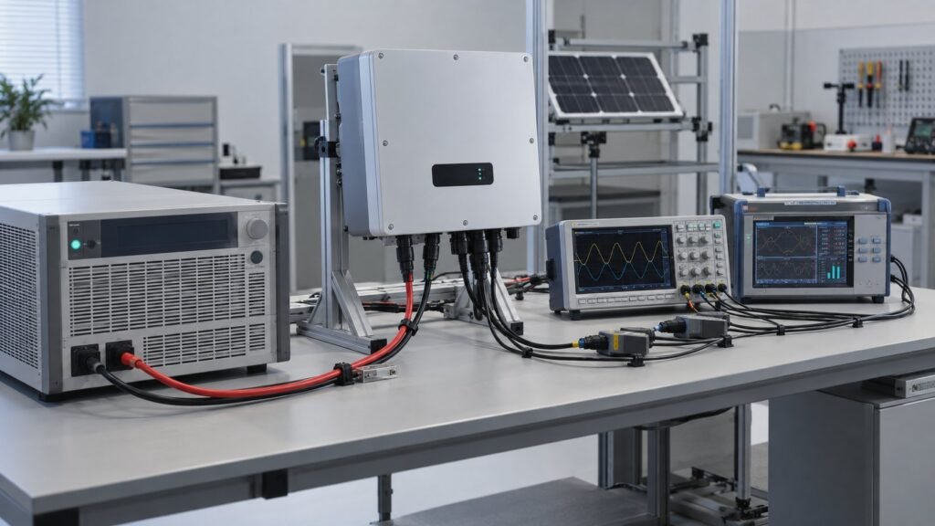
Solar array simulator MPPT testing is defensible when the source enforces a repeatable photovoltaic I-V curve, the wiring follows EN 50530 Clause 4.2, and every efficiency result records its measurement location, stabilisation period, curve, and uncertainty. A stiff DC supply cannot provide that evidence because it holds voltage instead of reproducing array behaviour.
The September 2026 GSAS article, Solar Array Simulation for PV Inverter MPPT Testing, defines the simulator correctly: it is a source that controls a soft photovoltaic I-V curve. Your acceptance method must then convert that capability into clause-based records that a certification laboratory can repeat.
What must solar array simulator MPPT testing prove?
Your simulator must make the inverter see a controlled PV characteristic, not a fixed 400 V bus. GSAS describes the soft curve as one where voltage changes as the inverter draws current. The curve includes open-circuit voltage, short-circuit current, and a defined maximum power point. That lets you repeat the same PV inverter MPPT test across firmware revisions.
Use a programmed curve with a documented PV model, irradiance, temperature, VMPP, IMPP, and P-MPP. For partial-shading work, record every local maximum and the global maximum. A current-limit clamp, flat voltage response, or undocumented curve invalidates the result because the inverter is no longer tracking the declared source.
See also: Battery Simulator for BMS Testing Under GB/T 47136
How should you wire the EN 50530 test setup?
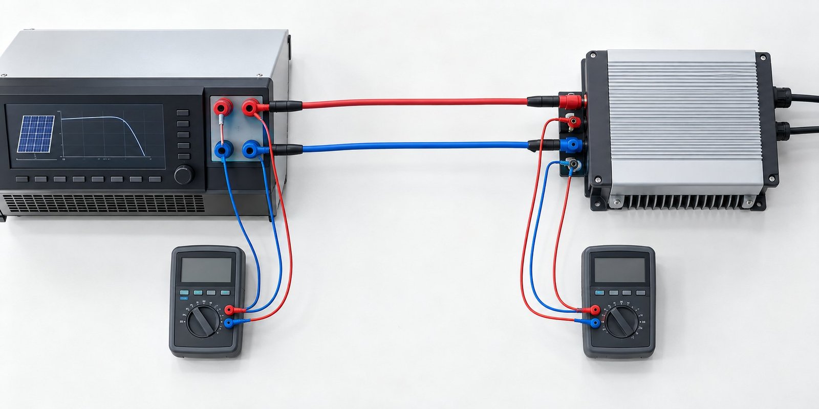
EN 50530:2010/A1:2013 Clause 4.2 separates the measurement points by purpose. Measure DC voltage close to the PV simulator for MPPT efficiency. Measure DC voltage close to the inverter terminals for conversion efficiency. For combined testing, measure both locations so cable voltage drop does not enter the calculation.
- Connect the simulator to the inverter DC input and route the inverter AC output to the laboratory grid interface or grid simulator. Failure mode: an undersized AC path limits inverter power and appears as poor MPPT performance.
- Install voltage sense points at the simulator terminals and DUT terminals. Failure mode: using only the simulator voltage hides cable drop and corrupts combined MPPT and conversion results.
- Set ambient temperature to 25 °C ±5 °C, or record the mutually agreed alternative in the report. Failure mode: an undocumented temperature prevents comparison between laboratories.
- Load the declared c-Si PV model and verify the curve before energising the inverter. Annex A.1 provides the PV-simulator requirements to check. Failure mode: an incorrect VMPP, IMPP, or irradiance setting changes the available power.
- After each power change, wait 2 minutes before evaluation. For each static condition, measure for 10 minutes. Failure mode: including settling data captures the inverter’s search transient instead of steady MPPT behaviour.
- Log PMPP,PVS, PDC, UMPP,PVS, IMPP,PVS, IDC, and PAC after tracking stabilises. Failure mode: missing source power or terminal voltage prevents an independent efficiency calculation.
How does EN 50530 define static and dynamic MPPT efficiency?
EN 50530 Clause 4.3 covers conversion and static MPPT efficiency with a fixed curve and defined power levels. Clause 4.4.1 covers dynamic MPPT efficiency with irradiance changes. The EN 50530 MPPT efficiency result is meaningful only when the source profile, model, measurement window, and logged quantities are retained with the report.
| Test | Standard condition | What you calculate | Failure mode and use when |
|---|---|---|---|
| Static MPPT | Fixed curve; 10-minute measurement window after stabilisation | ηMPPT,static = PDC ÷ PMPP,PVS × 100 | Fails the method if settling data is included; use for steady tracking accuracy. |
| Dynamic MPPT | Irradiance ramps from 100 to 500 W/m² with slopes from 0.5 to 50 W/m²/s | Dynamic tracking performance over the Annex B profile | Fails the profile if the source cannot reproduce the commanded slope; use for tracking during changing irradiance. |
| Combined conversion and MPPT | Voltage measured at both simulator and DUT terminals | MPPT and conversion results separated from cable loss | Fails traceability if one voltage location is assumed; use for certification evidence. |
Normative Annex B specifies the dynamic profiles. The 100–500 W/m² sequence uses ramp-up and ramp-down slopes from 0.5 to 50 W/m²/s. Repeat the sequence with the c-Si model required by Clause 4.4.1, document the PV technology, and identify whether the inverter loses the peak, oscillates around it, or recovers late.
Which simulator specifications support a defensible result?
Choose the source by its curve control, measurement path, and response time. Chroma’s Solar Array Simulator DC Power Supply page lists direct Voc, Isc, Vmp, and Imp programming, plus 128–4096-point user tables. That supports repeatable custom and shaded curves. Confirm that the exact model also meets your voltage and power envelope.
| Platform | Relevant capability | Use when |
|---|---|---|
| Chroma 62000H-S | Voc, Isc, Vmp, and Imp programming; 128–4096-point voltage/current tables; EN50530 and Sandia models | Use for parameter-driven curves, shadowed tables, and repeatable PV inverter verification. |
| Ultra N35500 with NS91000 | 360, 500, 750, 1000, 1500, and 2250 V classes; EN50530 and Sandia profiles; voltage rise/fall ≤5 ms; transient recovery below 4.5 ms from 10% to 60% | Use when your test bench needs high-power bidirectional operation and a dynamic MPPT test across string-inverter voltage classes. |
| Stiff programmable DC supply | Fixed-voltage or current-limit operation without a declared PV I-V curve | Use for DC bus or protection checks, not for defensible MPPT efficiency. |
The Ultra N35500 platform covers bidirectional and regenerative DC operation from 0–2250 V across six voltage classes, with representative 3U response figures of ≤5 ms rise/fall and less than 4.5 ms transient recovery from 10% to 60%. Its NS91000 software provides PV I-V/P-V simulation with EN50530 and Sandia profiles. See the NS91000 PV array simulation software specification when you define profile control and logging.
See also: MCS Charger Test Power Supply: What IEC TS 63379 Fixes
What should the measured acceptance record contain?
Record one result with the programmed curve, measured source values, DUT-terminal values, instrument uncertainty, and calculation. A worked Ultra N35500 and NS91000 static record at a nominal 1000 V, 10 A MPP illustrates the required format.
| Record field | Measured or declared value |
|---|---|
| Curve | c-Si static curve; nominal VMPP 1000 V, IMPP 10.000 A, PMPP 10.000 kW |
| Simulator terminals | 999.8 V and 10.004 A; measured PMPP,PVS = 10.002 kW |
| DUT terminals | 997.0 V and 9.970 A; measured PDC = 9.940 kW |
| Instrument uncertainty | Ultra voltage readback ≤ ±0.4 V at 1000 V full scale; external DC power meter ±0.10% of reading |
| Calculated static efficiency | ηMPPT,static = 9.940 ÷ 10.002 × 100 = 99.38% |
Treat 99.38% as a measured result for the declared conditions, not as a universal EN 50530 pass line. Your laboratory or customer must define the acceptance limit. At a 99.0% limit this record passes; at 99.5% it fails. Include the uncertainty budget, curve file, calibration status, and raw 10-minute data in the report.
For the complete PV inverter test power supply workflow, keep the DC source, AC path, measurement instruments, and protection limits under one test revision. Ashkan, power supply engineer at Ultra Power Systems, specifies the source and measurement chain together because a fast curve without traceable logging does not make a defensible result.
Solar array simulator MPPT testing FAQ
Is EN 50530 a pass or fail limit?
EN 50530 defines the measurement method and test conditions. Your certification programme, customer specification, or procurement document must define the acceptance threshold.
Where should you measure DC voltage?
Measure close to the PV simulator for MPPT efficiency. Measure close to the inverter for conversion efficiency. Use both locations for combined measurements.
Why does a dynamic MPPT test need response-time evidence?
The source must change its I-V curve at the commanded irradiance slope. If its response is slower than the profile, the source becomes part of the error and the inverter result cannot be isolated.
Make the simulator part of the evidence trail
A defensible PV inverter result is a chain: soft I-V curve, Clause 4.2 wiring, Annex A.1 simulator checks, 2-minute stabilisation, 10-minute static windows, Annex B ramps, terminal measurements, and uncertainty. If your bench needs 360–2250 V operation with EN50530/Sandia profiles, review the solar array simulator DC power supply for PV inverter MPPT testing and define the acceptance record before ordering →
What uncertainty should an EN 50530 MPPT test report include?
An EN 50530:2010/A1:2013 report should state MPPT efficiency with expanded uncertainty U using coverage factor k=2, including voltage, current, power, timing, and cable-drop contributions.
Use calibration certificates traceable to ISO/IEC 17025 for each measurement channel, and state the sample count used for the result—for example, 600 one-second samples over a 10-minute window. Keep simulator-setting tolerance separate from instrument uncertainty and propagate measured simulator-to-DUT voltage drop into the final value.